Definition 2.1. Two events (elements of \(\mathcal{F}\)) \(A\) and \(B\) are independent if \(P(A \cap B) = P(A) P(B)\).

Definition 2.2. Two random variables \(X\) and \(Y\) are independent if for all \(C, D \in \mathcal{B}_{\mathbb{R}}\),

Definition 2.3. Two (sub)\(\sigma \)-algebras (of \(\mathcal{F}\)) \(\mathcal{F}_1\) and \(\mathcal{F}_2\) are independent if for all \(A \in \mathcal{F}_1\) and \(B \in \mathcal{F}_2\), the events \(A\) and \(B\) are independent.

Theorem 2.4.

1.

If \(X\) and \(Y\) are independent r.v.’s then so are \(\sigma (X)\) and \(\sigma (Y)\).

2.

Conversely, if \(X\), \(Y\) are r.v.’s, \(\mathcal{F}_1\) and \(\mathcal{F}_2\) are independent, \(X\) is \(\mathcal{F}_1\)-measurable and \(Y\) is \(\mathcal{F}_2\)-measurable, then \(X\) and \(Y\) are independent.

Theorem 2.5.

1.

If \(A\) and \(B\) are independent, then so are \(A^c\) and \(B\), \(A\) and \(B^c\), and \(A^c\) and \(B^c\).

2.

Events \(A\) and \(B\) are independent iff \(1_A\) and \(1_B\) are independent.

Definition 2.6. \(\sigma \)-algebras \(\mathcal{F}_1, \mathcal{F}_2, \ldots , \mathcal{F}_n\) are independent if whenever \(A_i \in \mathcal{F}_i\) for \(i = 1, \ldots , n\), we have

\[ P\left (\bigcap _{i=1}^n A_i\right ) = \prod _{i=1}^n P(A_i) \]

Definition 2.7.

Random variables \(X_1, \ldots , X_n\) are independent if whenever \(B_i \in \mathcal{B}_\mathbb{R}\) for \(i = 1, \ldots , n\), we have \[ P\left (\bigcap _{i=1}^n X_i^{-1}(B_i)\right ) = \prod _{i=1}^n P(X_i \in B_i) \]

Definition 2.8.

Sets \(A_1, \ldots , A_n\) are independent if whenever \(I \subset \{1, \ldots , n\}\), we have \[ P\left (\bigcap _{i \in I} A_i\right ) = \prod _{i \in I} P(A_i) \]

Lemma 2.9. If \(A_1, \dots , A_n\) are independent then so are \(A_1^c, \dots , A_n\).

Theorem 2.10. Events \(A_1, \dots , A_n\) are independent iff \(1_{A_1}, \dots , 1_{A_n}\) are independent.

Theorem 2.11. Random variables \(X_1, \dots , X_n\) are independent iff \(\sigma (X_1), \dots , \sigma (X_n)\) are independent.

Remark 2.12. Pairwise independence is NOT the same as independence.

Definition 2.13. Events \(A_1, A_2, \dots \) are independent if for all finite positive integer sequence \(s_1, \dots , s_n\) the events \(A_{s_1}, \dots , A_{s_n}\) are independent. We define independece for random variables and sigma algebras analogously.

Theorem 2.14. Events \(A_1, A_2, \dots \) are independent iff r.v.’s \(1_{A_1}, 1_{A_2}, \dots \) are independent.

Theorem 2.15. Random variables \(X_1, X_2, \dots \) are independent iff \(\sigma (X_1), \sigma (X_2), \dots \) are independent.

Definition 2.16.

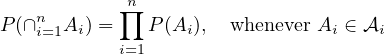
Collections of sets \(\mathcal{A}_1, \dots , \mathcal{A}_n \subset \mathcal{F}\) are said to be independent if whenever \(A_i \in \mathcal{A}_i\) and \(I \subset \{1, \dots , n\}\) we have \(P(\cap _{i \in I} A_i) = \prod _{i \in I} P(A_i)\). We define independence for a countable collection of subsets of \(\mathcal{F}\) the same way we did in the previous subsection.

Remark 2.17. If \(\mathcal{A}_i = \{A_i\}\) this is the same as independence for events.

If each of the \(\mathcal{A}_i\) is a sub-\(\sigma \)-algebra of \(\mathcal{F}\), this is the same as independence for \(\sigma \)-algebras.

Lemma 2.18. If \(\Omega \in \mathcal{A}_i\), we can reduce the condition of independece to

Definition 2.19. \(\mathcal{A} \subset \mathcal{P}(\Omega )\) is a \(\pi \)-system if it is non-empty and closed under (finite) intersection.

Definition 2.20. \(\mathcal{L} \subset \mathcal{P}(\Omega )\) is a \(\lambda \)-system if

1.

\(\Omega \in \mathcal{L}\)

2.

\(A, B \in \mathcal{L}\) and \(A \subset B\) implies \(B \setminus A \in \mathcal{L}\)

3.

If \(A_n \in \mathcal{L}\), \(A_n \subset A_{n+1}\), \(A = \cup _{i=1}^n A_i\) then \(A \in \mathcal{L}\).

Theorem 2.21 (Dynkin’s \(\pi \)-\(\lambda \) theorem). If \(\mathcal{P}\) is a \(\pi \)-system and \(\mathcal{L}\) is a \(\lambda \)-system that contains \(\mathcal{P}\) then \(\sigma (\mathcal{P}) \subset \mathcal{L}\).

Theorem 2.22. Suppose \(\mathcal{A}_1, \dots , \mathcal{A}_n\) are independent and each of them is a \(\pi \)-system. Then \(\sigma (\mathcal{A}_1), \dots , \sigma (\mathcal{A}_n)\) are independent.

Corollary 2.23. The same holds for a countable sequence of independent \(\pi \)-systems \(\mathcal{A}_1, \mathcal{A}_2, \dots \).

Corollary 2.24. Theorem 2.22 holds for any countable set of random variables (the product may be infinite).

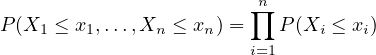
Theorem 2.25. In order for \(X_1, \dots , X_n\) to be independent, it is sufficient that for all \(x_i \in (-\infty , \infty ]\).

Theorem 2.26. Suppose \(\mathcal{F}_{i, j}\), \(1 \leq i \leq n\), \(1 \leq j \leq m(i)\) are independent sub-\(\sigma \)-algebras of \(\mathcal{F}\) and let \(\mathcal{G}_i = \sigma (\cup _j \mathcal{F}_{i, j})\). Then \(\mathcal{G}_1, \dots , \mathcal{G}_n\) are independent.

Corollary 2.27. The previous theorem holds for a countable number of families \(\sigma \)-algebras, each with a countable number of members.

Theorem 2.28. if for \(1 \leq i \leq n\), \(1 \leq j \leq m(i)\), \(X_{i, j}\) are independent and \(f_i : \mathbb{R}^{m(i)} \to \mathbb{R}\) are measurable then \(f_i(X_{i, 1}, \dots , X_{i, m(i)})\) are independent.

Corollary 2.29. The previous theorem also applies to a countable set of finite families of random variables.

Theorem 2.30. If \(X_1, \dots , X_n\) are random variables and \(X_i\) has distribution \(\mu _i\), then \((X_1, \dots , X_n)\) has distribution \(\mu _1 \times \dots \times \mu _n\).

Theorem 2.31. Suppose \( X \) and \( Y \) are independent and have distributions \( \mu \) and \( \nu \). If \( h : \mathbb{R}^2 \to \mathbb{R} \) is a measurable function with \( h \geq 0 \) or \( E|h(X, Y)| < \infty \), then \[ E h(X, Y) = \int \int h(x, y) \, \mu (dx) \, \nu (dy). \]

In particular, if \( h(x, y) = f(x) g(y) \) where \( f, g : \mathbb{R} \to \mathbb{R} \) are measurable functions with \( f, g \geq 0 \) or \( E|f(X)| \) and \( E|g(Y)| < \infty \), then \[ E f(X) g(Y) = E f(X) \cdot E g(Y). \]

Theorem 2.32. If \( X_1, \dots , X_n \) are independent and have (a) \( X_i \geq 0 \) for all \( i \), or (b) \( E|X_i| < \infty \) for all \( i \), then \[ E \left ( \prod _{i=1}^n X_i \right ) = \prod _{i=1}^n E X_i \] i.e., the expectation on the left exists and has the value given on the right.

Definition 2.33. Two random variables \(X\) and \(Y\) with \(EX^2 < \infty \), \(EY^2 < \infty \) that have \(E(XY)=EXEY\) are said to be uncorrelated. The finite second moments are needed so that we know \(E|XY| < \infty \) by the Cauchy-Schwarz inequality.

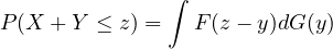
Theorem 2.34. If \(X\) and \(Y\) are independent, \(F(x) = P(X \leq x)\), and \(G(y) = P(Y \leq y)\), then

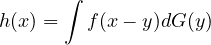
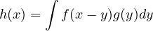
Theorem 2.35. Suppose that \(X\) with density \(f\) and \(Y\) with distribution function \(G\) are independent. Then \(X+Y\) has density

Example 2.36. The gamma density with parameters \( \alpha \) and \( \lambda \) is given by \[ f(x) = \begin{cases} \frac{\lambda ^\alpha x^{\alpha -1} e^{-\lambda x}}{\Gamma (\alpha )} & \text{for } x \geq 0, \\ 0 & \text{for } x < 0, \end{cases} \] where \( \Gamma (\alpha ) = \int _0^\infty x^{\alpha -1} e^{-x} \, dx \).

Theorem 2.37. If \( X = \text{gamma}(\alpha , \lambda ) \) and \( Y = \text{gamma}(\beta , \lambda ) \) are independent, then \( X + Y \) is \( \text{gamma}(\alpha + \beta , \lambda ) \). Consequently, if \( X_1, \dots , X_n \) are independent exponential(\( \lambda \)) random variables, then \( X_1 + \cdots + X_n \) has a gamma(\( n, \lambda \)) distribution.

Example 2.38. Normal density with mean \(\mu \) and variance \(\sigma ^2\): \[ (2\pi \sigma ^2)^{-1/2} \exp \left (-\frac{(x - \mu )^2}{2\sigma ^2}\right ). \]

Theorem 2.39. If \(X \sim \operatorname{normal}(\mu , a)\) and \(Y \sim \operatorname{normal}(\nu , b)\) are independent then \(X + Y \sim \operatorname{normal}(\mu + \nu , a + b)\).

Theorem 3.1 (Kolmogorov’s Extension Theorem). Suppose we are given probability measures \(\mu _n\) on \((\mathbb{R}^n, \mathcal{B}_{\mathbb{R}^n})\) that are consistent, that is,

Definition 3.2. \((S, \mathcal{S})\) is said to be a standard Borel space if there is a \(1-1\) map \(\varphi \) from \(S\) into \(\mathbb{R}\) so that \(\varphi \) and \(\varphi ^{-1}\) are both measurable.

Theorem 3.3. If \(S\) is a Borel subset of a complete separable metric space \(M\), and \(\mathcal{S}\) is the collection of Borel subsets of \(S\), then \((S, \mathcal{S})\) is a standard Borel space.

Definition 4.1. \(Y_n\) converges in probability to \(Y\) if for all \(\epsilon > 0\), \(P(|Y_n - Y| > \epsilon ) \to 0\) as \(n \to \infty \).

Definition 4.2.

A family of random variables \(X_i\) (\(i \in I\)) with \(EX_i^2 < \infty \) is said to be uncorrelated if we have

Theorem 4.3. Let \(X_1, \dots , X_n\) have \(EX_i^2 < \infty \) and be uncorrelated. Then

Lemma 4.4. If \(p > 0\) and \(E|Z_n|^p \to 0\) then \(Z_n \to 0\) in probability.

Theorem 4.5 (\(L^2\) weak law). Let \(X_1, X_2, \dots \) be uncorrelated random variables with \(EX_i = \mu \) and \(\operatorname{var}(X_i) \leq C < \infty \). If \(S_n = X_1 + \dots + X_n\) then as \(n \to \infty \), \(S_n/n \to \mu \) in \(L^2\) and in probability.

Definition 4.6. When \(X_1, X_2, \dots \) are all independent random variables with the same distributon, we say they’re independent and identically distributed (i.i.d.).

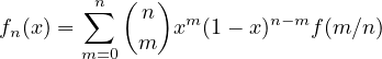
Example 4.7 (Polynomial approximation). Let \(f\) be a continuous function on \([0, 1]\), and let

Example 4.8 (A high-dimensional cube is almost the boundary of a ball). Let \(A_{n, \varepsilon } = \{x \in \mathbb{R}^n : (1 - \varepsilon ) \sqrt{n/3} < |x| < (1 + \varepsilon ) \sqrt{n/3} \}\). Then for any \(\varepsilon > 0\), \(|A_{n, \varepsilon } \cap (-1, 1)^n| / 2^n \to 1\).

Theorem 4.9. (Here \(X_{n, 1}, \dots , X_{n, n}\) can be any sequence of random variables) Let \(\mu _n = ES_n\), \(\sigma _n^2 = \operatorname{var}(S_n)\). If \(\sigma _n^2/b_n^2 \to 0\) then

Definition 4.10. To truncate a random variable at level \(M\) means to consider

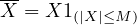
Theorem 4.11 (Weak law for triangular arrays). For each \(n\), let \(X_{n, k}\) (\(1 \leq k \leq n\)) be independent. Let \(b_n > 0\) with \(b_n \to \infty \), and let \(\overline{X}_{n, k} = X_{n, k} 1_{(|X_{n, k}| \leq b_n)}\). Suppose that as \(n \to \infty \)

1.

\(\sum _{k=1}^n P(|X_{n, k}| > b_n) \to 0\) and

2.

\(b_n^{-2} \sum _{k=1}^n E \overline{X}_{n, k}^2 \to 0\)

If we let \(S_n = X_{n, 1} + \dots + X_{n, n}\) and put \(a_n = \sum _{k=1}^n E \overline{X}_{n, k}\), then

Theorem 4.12 (Weak law of large numbers). Let \(X_1, X_2, \dots \) be i.i.d. with

Lemma 4.13. If \(Y \geq 0\) and \(p > 0\) then \(E(Y^p) = \int _0^\infty p y^{p-1} P(Y > y) dy\).

Remark 4.14. Taking \(p = 1 - \varepsilon \) here shows that \(xP(|X_1| > x) \to 0\) implies \(E|X_1|^{1- \varepsilon } < \infty \). This means that the assumption made in the previous theorem is not much weaker than finite mean.

Theorem 4.15. Let \(X_1, X_2, \dots \) be i.i.d. with \(E|X_i| < \infty \) and let \(S_n = X_1 + \dots + X_n\) and let \(\mu = EX_1\). Then \(S_n/n \to \mu \) in probability.

Exercise 5.1. Prove that \(P(\limsup A_n) \geq \limsup P(A_n)\) and \(P(\liminf A_n) \leq \liminf P(A_n)\).

Definition 5.2. It is common to write \(\limsup A_n = \{ \omega : \omega \in A_n \text{ i.o.} \}\) where i.o. means infinitely often.

Theorem 5.3 (Borel-Cantelli lemma). If \(\sum _{n=1}^\infty P(A_n) < \infty \) then \(P(A_n \text{ i.o.}) = 0\) (in the sense of \(P(\limsup A_n)=0\)).

Theorem 5.4. \(X_n \to X\) in probability iff for every subsequence \(X_{n(m)}\) there is a further subsequence \(X_{n(m_k)}\) that converges a.s. to \(X\).

Theorem 5.5. If \(f\) is continuous and \(X_n \to X\) in probability then \(f(X_n) \to f(X)\) in probability. If, in addition, \(f\) is bounded then \(Ef(X_n) \to Ef(X)\).

Theorem 5.6. If \(X_1, X_2, \dots \) are i.i.d. with \(EX_i \to \mu \) and \(EX_i^4 < \infty \) and \(S_n = X_1 + \dots + X_n\) then \(S_n/n \to \mu \) a.s.

Theorem 5.7 (The second Borel-Cantelli lemma). If the events \(A_n\) are independent then \(\sum P(A_n) = \infty \) implies \(P(\limsup A_n) = 1\).

Theorem 5.8. If \(X_1, X_2, \dots \) are i.i.d. with \(E|X_i| = \infty \), then \(P(|X_n| \geq n \text{ i.o.}) = 1\). So if \(S_n = X_1 + \dots + X_n\) then \(P(\lim S_n/n \text{ exists and } \in (-\infty , \infty )) = 0\).

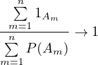
Theorem 5.9. If \(A_1, A_2, \dots \) are pairwise independent and \(\sum _{n=1}^\infty P(A_n) = \infty \), then as \(n \to \infty \)

Theorem 5.10. Let \(X_1, X_2, \dots \) be pairwise independent identically distributed random variables with \(E|X_i| < \infty \). Let \(EX_i = \mu \) and \(S_n = X_1 + \dots + X_n\). Then \(S_n/n \to \mu \) a.s. as \(n \to \infty \).